

|
|
Terrain roughnessTerrain roughness of the sea floor influences the tides, currents and waves, modifying hydrodynamics and aerodynamics and creating sheltered areas in the wake of elevated terrain[26]. ‘Sticky water’ is the name of the effect where water slows down, appearing to cling to the rough surfaces and crannies, enabling pelagic larvae of fish and corals near coral reefs to persist close to their source and/or settle[1]. Quick facts
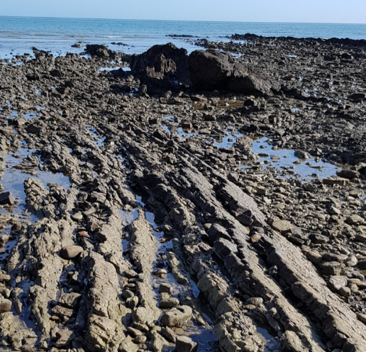
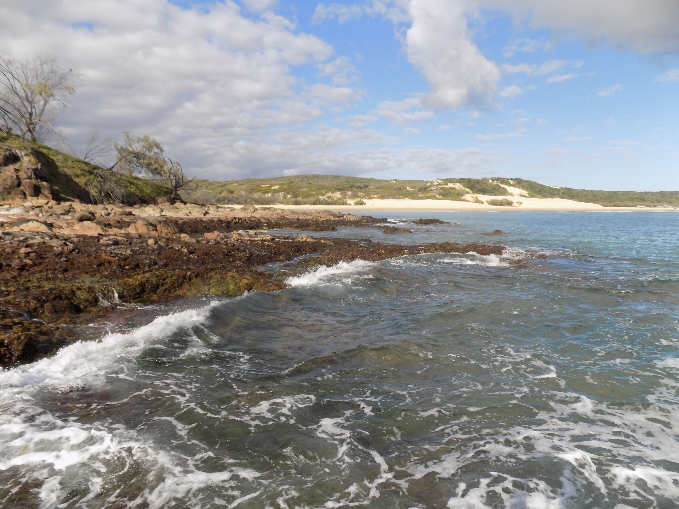
Why is terrain roughness important?Terrain roughness, which characterises variability or irregularity in elevation within a spatial unit, needs to be considered with other terrain attributes such as relative relief. It is critical to clearly define the scale or level at which terrain roughness is being considered, and the unit which is being used to measure across a ‘window’ of scale, as different attributes will be relevant at different scales[13][22]. In earth sciences, spatial variations in surface roughness are used to delineate landform components and infer process information to derive geomorphological units. Roughness of the subtidal sea floor and intertidal area is important for providing variation in biophysical components, patterns and processes. It provides for habitat complexity and heterogeneity, and high terrain roughness is often an indicator of high species-richness and biodiversity hot spots at a range of scales[17]. Subtidally, terrain roughness influences energy flows (current speed, wave energy and direction), sediment grain size, and water column circulation and nutrients dynamics, leading to higher water column productivity, benthic biomass and species diversity[28]. Areas of high terrain variability contribute to a diversity of oceanographic processes, such as upwelling of nutrients within canyons and along continental shelf margins[11]. High sea floor heterogeneity can be indicative of features such as rocky reefs, mesophotic reefs, carbonate mounds, pock-marks (submarine groundwater discharge) and in the absence of biota inventory, can be used to predict the distribution of benthic fauna[21][25]. Intertidally, roughness influences: aerodynamic flow and evaporation; hydrodynamic flows, including surface and ground water movement, runoff and infiltration; geomorphological processes, such as sediment transport and bank erosion; and chemical processes such as redox conditions, oxygen penetration and nutrient availability[22]. Many different geomorphological and geological processes have contributed, over time and at different scales, to produce different degrees of roughness on the sea floor and in intertidal area. Around 140 million years ago continental drift began to break the plates of the earth’s crust apart, and the continental slopes and sea floor elevated plateaux (e.g. the Queensland Plateau, formed around 60 million years ago) mark the regional scale boundaries of these original plates[16]. The continental shelf is not always smooth at the subregional scale. Over the various glacial-interglacial cycles, the present continental shelf was exposed as land, where old river valleys weathered deeper channels and depressions. During the ice ages, today’s coral reefs were limestone hills on the alluvial plains, and coral reefs grew along the shelf edge and upper margins of the present day continental slope[24]. Today rougher areas on digital bathymetry predict locations of these mesophotic reefs[3]. Past sedimentary processes, faulting and folding, volcanic activity, erosion and deposition have all contributed to the roughness of today’s sea floor and intertidal area. For example, the roughness of present-day rocky shorelines is a product of the interaction between wave energy and lithology[27]. Usually greater sea floor roughness is associated with a consolidated substrate, although heterogeneous patterns associated with submerged dunefields and sandbanks may also be present and can reflect old aeolian processes or present-day tidal currents[21][22]. Examples of intertidal and subtidal scale consideration, with related biophysical attributes:
At the sub-regional scale, coral reef systems provide more terrain roughness than non-reefal areas, and this in turn, significantly alters hydrodynamic energy (i.e. waves and currents)[1]. Measuring terrain roughnessThere are a number of different ways to measure terrain roughness (metrics), and different mapping surrogates from which to extract these metrics. Traditionally, roughness was measured along a straight line using a chain draped over the terrain. Nowadays, it is more often derived from a Digital Terrain Model (DTM), which measures the height of a surface from a vertical datum and is a three-dimensional model consisting of x, y (area) and z (elevation/depth) coordinates. Some metrics of terrain roughness gauge how different the terrain varies across three dimensions when compared with an equivalent two-dimensional flat area[10][8]. In general, the terrain roughness measures how much the z-axis varies, within a defined area at a defined scale, across the sampled area of terrain. A DTM represents highs and lows from which roughness can be measured or characterised, including topographic features (i.e. geomorphology) based on relief and morphology. A DTM can be produced from a variety of field methods (e.g. multi-beam echosounders - MBES, LiDAR systems), and can be used to derive sea floor terrain attributes that can serve as mapping surrogate dataset. For example, backscatter data from MBES can provide a measure of roughness.
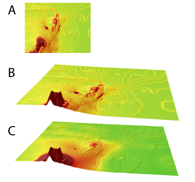
Three views of Terrain Ruggedness Index (TRI), showing the effect of scale on the calculation. A): and B): 3 X 3 TRI picks out many different fine-scale features. This is a window of calculation of 90m i.e. three pixels of the 30m DEM. C): 10 X 10 TRI picks out major ridges at a broader scale and misses finer features, while attributing ruggedness to a wider area than the 3 X 3 calculation. The window of calculation is 300m. Calculated from the CEQ30 DEM (DES, 2019) in SAGA-GIS[4] Module Terrain Ruggedness Index[19]
Roughness metrics calculated from DTMs are available either as stand-alone, or embedded in packages of terrain derivative tools. Several stand-alone metrics use the size of a ‘moving window’ and are scale or slope dependent. Some metrics include: (i) Vector ruggedness measures (VRM) capture variability in slope and aspect in a single ratio[20][9]. The various VRMs available tend to produce similar outputs[14]. (ii) Terrain Ruggedness Index calculates the sum change in elevation between a central cell and its eight surrounding neighbours, or a nominated number of adjacent cells[19]. Like most roughness metrics, TRI is scale-dependent as illustrated in the figure above which compares TRI calculated for 3 surrounding cells with that of 10 surrounding cells. (iii) Local standard deviations of elevation measures the departure of a pixel from the mean elevation, compared with its range[2]. Other metrics include: Surface Ratio, Melton Ruggedness Index, Roughness and Range[15], area ratio, vector dispersion, standard deviation of residual topography (SDrestopo), standard deviation of elevation (SDelev), standard deviation of slope (SDslope) and standard deviation of profile curvature (SDprofc)[9], arc-chord ratio[5]. Various roughness/terrain rugosity measures can be used in combination with other terrain indices to identify consolidated (hard) substrate[6]. Fractal dimension is a geometrical concept and index of complexity that compares how the roughness, regularity and detail of a pattern changes with the scale at which it is measured. The difference between fractal dimension and other measures of roughness is that it also considers how the roughness pattern changes at different hierarchical scales, and the degree of repetition of the patterns within patterns[25]. A consideration of roughness across different scales may be more appropriate to the attribute terrain pattern. Terrain derivative packages can include roughness metrics for semi-automated terrain mapping, for example:
Queensland Intertidal and Subtidal Classification SchemeFor the Intertidal and Subtidal Classification Scheme, the scale or level needs to be determined by the size or features of interest and the purpose of classification. The classification and mapping of Central Queensland did not use the attribute of roughness. Regardless of which metric or combinations of metrics are selected, roughness metrics selected at a specific scale will need to be reclassified into the categories of the scheme as suggested below. Where classified at a range of different scales, these should be nested hierarchically one within the other.
References
Last updated: 22 July 2020 This page should be cited as: Department of Environment, Science and Innovation, Queensland (2020) Terrain roughness, WetlandInfo website, accessed 25 June 2024. Available at: https://wetlandinfo.des.qld.gov.au/wetlands/ecology/aquatic-ecosystems-natural/estuarine-marine/itst/terrain-roughness/ |
Site footer

 — Department of Environment, Science and Innovation